Sparse Tensor-based Point Cloud Attribute Compression Using Augmented Normalizing Flows

 

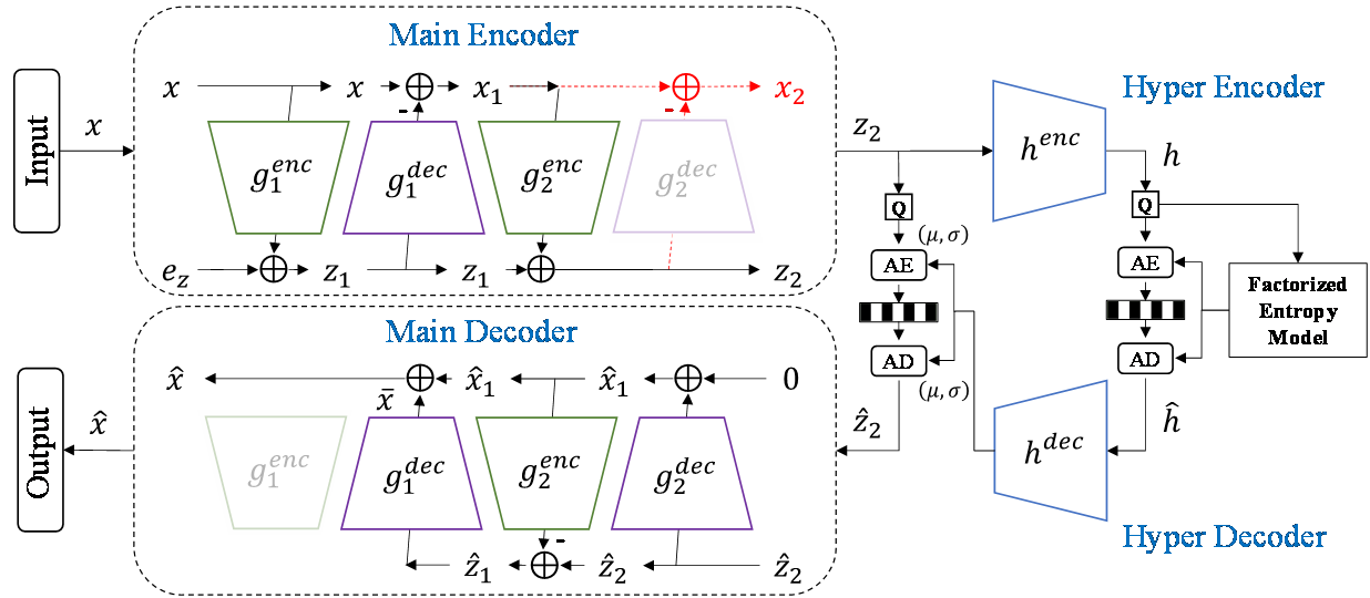
Fig. 1. The network architecture of our proposed ANF-PCAC. The red lines indicate the paths used during the training phase.

 

 

ABSTRACT

 

　The large amount of data of point cloud poses challenges for efficient storage and transmission. To address this problem, various learning-based techniques, in addition to rule-based solutions, have been developed for point cloud compression. While many previous works employed the variational autoencoder (VAE) structure, they have failed to achieve promising performance at high bitrates. We propose a novel point cloud attribute compression technique based on the Augmented Normalizing Flow (ANF) model, which incorporates sparse convolutions where a sparse tensor is used to represent the point cloud attribute. The invertibility of the NF model provides better reconstruction compared to VAE-based coding schemes. ANF provides a more flexible way to model the input distribution by introducing additional conditioning variables into the flow. Not only comparable to G-PCC, the experimental results demonstrate the effectiveness and superiority of the proposed method over several learning-based point cloud attribute compression techniques, even without requiring sophisticated context modeling.

 

PROPOSED METHOD

 

　The sparse convolution takes into account sparsity in CNNs by only computing outputs on predefined voxels and storing them as compact sparse tensors. It is efficient for irregular point clouds and can significantly reduce computation and memory costs. In our proposed network, we use sparse convolution as the basic operation. The sparse tensor   is represented by a set of coordinates    of the point cloud and the corresponding features , where   is the total number of occupied points. We assume that the point cloud geometry is available and can be losslessly coded, which is consistent with other learning-based point cloud attribute compression methods. In the following, we introduce our ANF model and the internal VAE structure in detail, as well as our training strategy.

 

A. ANF-PCAC

 

Following the design in ANFPCGC, we proposed ANF-based point cloud attribute compression. Fig. 1 shows the network architecture of the proposed ANF-PCAC, which is built upon SparsePCAC while discarding the context model. ANF-PCAC consists of two parts: the main encoder/decoder and the hyper encoder/decoder. We employ two layers of autoencoding transform in the main encoder/decoder, resulting in a two-step ANF that balances model capacity and complexity. The two autoencoding transforms have the same design with  and  sharing the same structure, and so do  and . In  and , we perform the reverse operation to reconstruct the point cloud attributes. 

 

During encoding, we input the point cloud attribute and an augmented noise  which follows a Gaussian distribution with zero mean. In the experiments,  is set to zero. During the training, we obtain an additive coupling output  by feeding the input to the first encoding transform . Then we get the difference between x and the reconstructed one, denoted as  after performing the first decoding transform  In the next step,   and  are served as inputs to the second autoencoder, and we get  and  as the final output of the main encoder, as shown in (1) and (2):

 

 )                                                                                      (1)

 )                                                                                      (2)

 

As indicated in (2),  is the difference between the original  and the reconstructed one and is expected to be close to zero if the encoding and decoding are well matched to each other. It implies that the input information  is expected to be completely transferred to the latent   It this way, we can save bits if   is not transmitted. In inference,  is not executed during encoding.

 

　After quantization, we perform decoding by reversing the operation of encoding. Following the design in ANFPCGC, we do not transmit   and the main decoder performs reconstruction by setting   to zero. To reduce the mismatch between the true value of  and zero. We encourage   to be close to zero by including a loss term. We obtain   by feeding the quantized   to   Then we input    and   to the bottom autoencoder in a reverse direction, and we obtain the final output , as shown in (3)(4):

 

                                                                                              (3)

                                                                                                              (4)

 

To further reduce bit consumption, we use a conditional entropy model based on hyperpriors . The hyper encoder learns the probability distribution of the latent  and generates a hyper prior , which is then quantized as  and described by a factorized entropy model. Then  passes through the hyper decoder to generate the mean and variance  which are used to describe the distribution of the latent  With this conditional Gaussian distribution, the bits consumption of the latent  can be estimated.

B. Training strategy

 

To train the proposed ANF-PCAC, we use Lagrangain loss, as shown in (5). For the rate, there are two terms, denoted as   and  , presenting the rate of the latent  and the hyperprior  , respectively. Three terms are involved in the computation of the distortion. The first term    computes the mean squared error (MSE) between the input   and the reconstructed signal. The second term  measures the MSE between the input  and  with the aim of enabling better reconstruction for the autoencoding. As mentioned earlier,  represents the residual information that is expected to be approximated by zero. This task can be accomplished by including the third term.

 

                                                       (5)

 

EXPERIMENTAL RESULTS 

 

In this section, we will provide the information of our training and testing datasets, as well as the anchor schemes. We will also describe our training details, followed by the presentation of quantitative and qualitative comparisons to demonstrate the superiority of our proposed method.

 

A. Dataset and Anchor

 

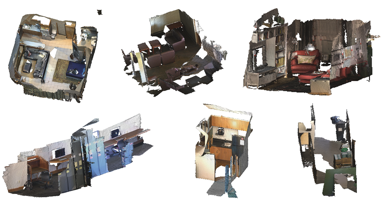
　For our training dataset, we utilize the ScanNet dataset, which is a large open-source dataset of indoor scenes. The dataset contains both high-quality and low-quality reconstructed meshes, and we used the high-quality version, as shown in Fig. 2. We converted the mesh into point cloud and scaled the geometry to 10 bits, followed by cube division with size   We randomly selected 50,000 cubes and used them for training. To make a fair comparison, the test dataset utilized in SparsePCAC  has been assessed. Four point clouds in the 8i Voxelized Full Body(8iVFB) are used, as shown in Fig. 3. Notably, our training and testing datasets are entirely different, enabling us to demonstrate the generalization ability of our proposed scheme. We compared our approach with three methods, including two learning-based methods: Deep PCAC and SparsePCAC, and a traditional point cloud compression standard G-PCC (TMC13v14).

 

B. Training Details

 

　We set to 0.05, 0.025, 0.01, 0.005, 0.0025, 0.001, 0.0005 and 0.00025 to obtain models with different bitrates.  is set as 0.01 to balance the distortion. We trained our models for 500 epochs, and all models use the initial learning rate  which gradually decreases to . We use Nvidia GeForce RTX 2080 Ti for training and testing.

C. Objective Quality Comparison

 

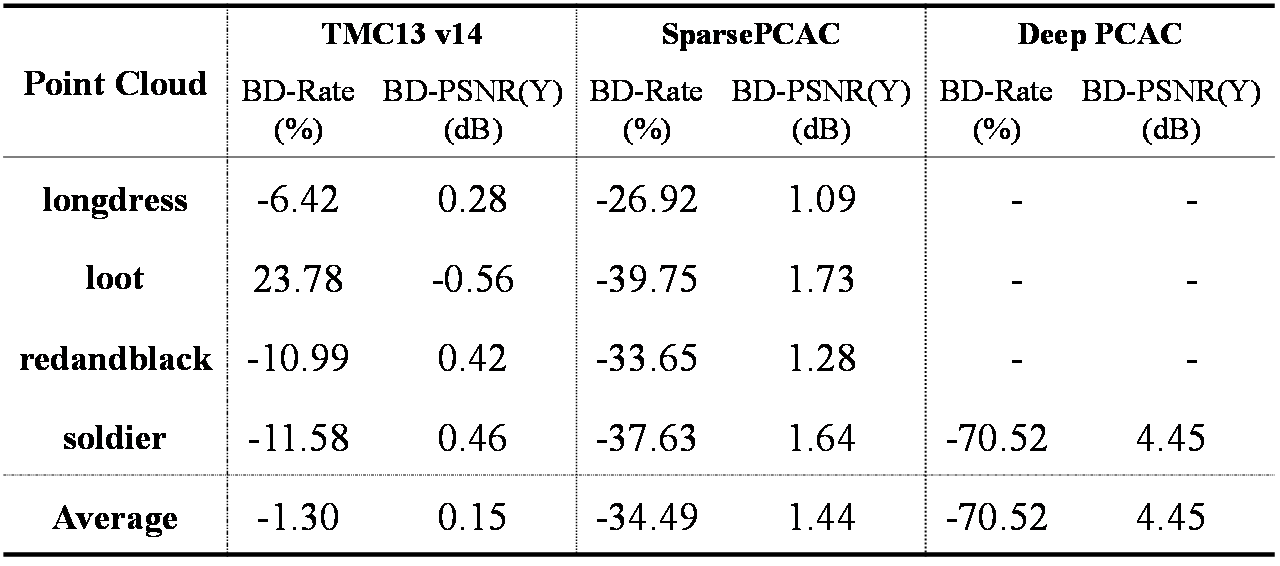
　We present the R-D (rate-distortion) performance in Fig.4, in which the bitrate is measured in bits per point (bpp) and the distortion is measured by the Peak Signal-to-Noise Ratio (PSNR) of the Y channel. Deep-PCAC evaluates only the sequence of soldiers in the 8iVFB dataset, while it is trained with others sequence in the same dataset. Fig. 4 shows that our proposed scheme outperforms Deep-PCAC and SparsePCAC. Additionally, our method is comparable with TMC13v14. To assess the average R-D performance, we used the Bjøntegaard metric, including BD-PSNR and BD-Rate, which is summarized in Table 1.  The results indicate that our method achieves, on average 70.52%, 34.49% and 1.3% rate reduction when compared to Deep PCAC, SparsePCAC and TMC13v14, respectively.

 

D. Runtime Comparison

 

　To specifically demonstrate the efficiency of our method where only a hyperprior is used to build the entropy model of the latent, we compare our method with SparsePCAC and TMC13v14. Since SparsePCAC relies on both autoregressive prior and hyperprior, it requires a more expensive inference time, as shown in Table 2.

 

Fig. 2: Training Dataset. Some high-quality version point cloud samples of ScanNet Dataset.

 

Fig. 3: Testing Dataset. 8iVFB dataset, from left to right are longdress, loot, redandblack, and soldier.

 

Fig. 4: R-D curves for longdress, loot, redandblack, and soilder.

 

 

Table 1: BD-Rate (%) and BD-PSNR (dB) with respect to anchor

 

 

Table 2: Average runtime for 8iVFB dataset