Point Cloud Geometry Compression Using Augmented Normalizing Flows
Chief investigator:
Siao-Yu Li, Jui-Chiu Chiang
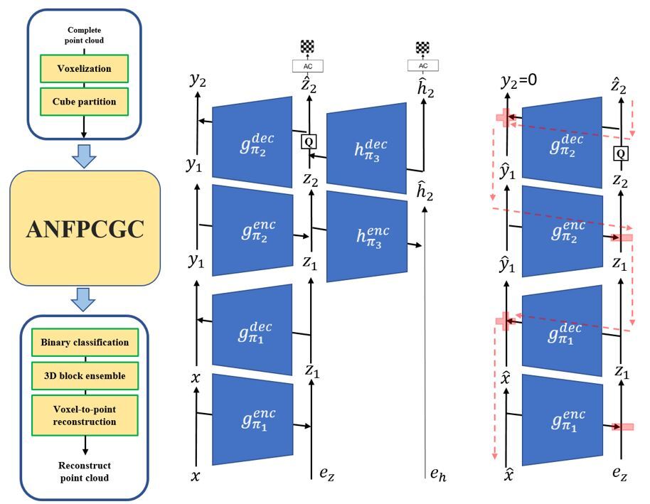
(a) Pipeline (b) Forward path (c) Backward path
Fig. 1. The proposed framework: (a) the main pipeline, (b) ANFPCGC in encoder mode (where the data flow from the bottom to the top as indicated by the black solid arrows), (c) ANFPCGC in decoder mode (where the data flow from the top to the bottom as indicated by the red dashed arrows).
ABSTRACT
With the increased popularity of immersive media, point clouds have become one of the popular data representations for presenting 3D scenes. The huge amount of point cloud data poses a great challenge on their storage and real-time transmission, which calls for efficient point cloud compression. This paper presents a novel point cloud geometry compression technique based on learning end-to-end an augmented normalizing flow (ANF) model to represent the occupancy status of voxelized data points. The higher expressive power of ANF than variational autoencoders (VAE) is leveraged for the first time to represent binary occupancy status. Compared to two coding standards developed by MPEG, namely G-PCC (geometry-based point cloud compression) and V-PCC (video-based point cloud compression), our method achieves more than 80% and 30% bitrate reduction, respectively. Compared to several learning-based methods, our method also yields better performance.
PROPOSED METHOD
In this section, we detail the proposed method. The proposed framework is shown in Fig. 1. It consists of a pre-processing module, the ANFPCGC codec, and a post-processing module.
A. Pre-processing
The pre-processing module aims to voxelize the input point cloud. A binary geometry representation then follows to indicate the occupancy status of every voxel, where 1 is assigned to the occupied voxel and 0 to the unoccupied one. Due to memory constraint during network training, the voxels are organized into non-overlapping 3D cubes of size 64×64×64, as shown in Fig. 1(a).
B. ANFPCGC Network Architectures
Figs. 1(b) and 1(c) show the network architecture of ANFPCGC. The left branch in Fig. 1(b) contains the autoencoding transforms for extracting the latent features. It stacks two layers of autoencoding transforms (i.e. two-step ANF) and forms a hierarchical ANF by including a hyperprior for the top layer, as illustrated on the right branch of Fig. 1(b). In theory, more layers of autoencoding transforms can be incorporated to gain higher expressive power. In practice, we choose two-step ANF, in order to strike a balance between the model capacity and complexity.
In ANFPCGC, every autoencoding transform is composed of a pair of the encoding and the decoding transforms, denoted as and
and
to be encoded, but also the augmented input
, which helps smoothly convert the input
into the latent space
through the autoencoding transforms. Ideally,
follows a Gaussian distribution with zero mean. However, for the sake of compression, we set
to zero, in order not to increase the entropy of the latent code
. The encoding and decoding for the hyperprior are specified by Eqs. (3) and (4), where the quantization
is performed by the nearest-integer rounding at inference time (and is modeled by an additive noise during training). Another augmented input
used for the hyperprior follows the uniform distribution between (-0.5, 0.5), i.e.,
Encoding transforms: (1)
Decoding transforms: (2)
Hyperprior encoding:  (3)
(3)
Hyperprior decoding:  (4)
(4)
With the augmented inputs ( ,
,
) , the encoding process of ANFPCGC is the composition of encoding transforms, decoding transforms, as well as the hyperprior encoding and decoding. That is,
where the encoding process starts from
and ends with
. After two-step ANF,
are obtained. But, only
are entropy encoded and transmitted. They are expected to capture as much information about the input
as possible. In the meantime,
is regularized to approximate a zero cube.
To reconstruct to 0. Despite the invertibility of ANF, there are two distortions introduced. The first is the quantization error on
and the other is the approximation error between the
produced by the encoding process and its approximate version, i.e. the zero cube, used in the decoding process. To reduce the impact of these errors, we adopt a quality enhancement module at the end of the backward path.
C. Post-processing
In post-processing, we perform the binary classification, 3D block ensemble and voxel-to-point reconstruction, as shown in Fig. 1 (a). First, the occupancy probability decoded by ANFPCGC needs to be binarized into 1 or 0 through the binary classification. The most simple and fast way is to set the threshold to be 0.5. But this classification strategy may impact considerably the rate-distortion (RD) performance, particularly due to the missing points. We thus adopt the adaptive threshold proposed in PCGCv1. The occupied voxel number m is signaled as side information. In the inference stage, the occupancy probability of each voxel in the 3D cube is sorted. Only the voxels with their occupied probabilities being among top-m are classified as 1, and the others as 0. After performing the binarization, all 3D cubes will be integrated into a complete voxelized point cloud. The final step is to describe the occupied voxel with its 3D coordinates to reconstruct the point cloud geometry.
D. Training objective
In training ANFPCGC, we use Lagrangian loss, as shown in Eq. (5), where the rate includes two terms (see Eq. (6)). They present the rate of the quantized hyperprior and the quantized latent
. Similar to [20],
and
are assumed to be a non-parametric distribution and a conditional Gaussian distribution, respectively.
(5)
(6)
D = {( FL) + (
Hierarchical FL) + (
) + (
)}} (7)
For the distortion, four terms are considered. The first term is the focal loss, which is used to address the unbalanced distribution of occupied and unoccupied voxels. The second term is called a hierarchical focal loss. It means we estimate also the occupancy status in the parent node. We take the advantage of the octree structure to gather both the information from nodes at the coarser level and the finest level. Fig. 3 shows an example where the left side is the parent and the children node for the input while the right side is the estimated occupancy status of the children and the corresponding parent node. This supplementary hierarchical focal loss leverages the closely connected information between the parent and the children nodes, and introduces a consistency constraint to help the network learn a better distribution.
Since we expect the information of the input to be well preserved in the latent space , the third term in (7) resolves the problem that
is not transmitted and is set to zero during decoding. Hence, with this loss, the network is learned to produce
with a value as close to zero as possible. Furthermore, not only
, but the output in the first ANF,
, should be close to zero during encoding by introducing the last loss term.

Fig. 3. Illustration of hierarchical focal loss
EXPERIMENTAL RESULTS
Datasets and training details:
Our training samples are randomly selected from ShapeNet [22], where the point clouds are partitioned into 3D cubes of size 64´64´64. For testing, four point clouds in the 8i Voxelized Full Bodies (8iVFB) dataset [23] are used, including longdress_vox10_1300,loot_vox10_1200, solider_vox_0690 and redandblack_vox10_1550, which are selected as the test set 1 by MPEG AI-3DGC [24]. They are full-body point clouds with dense samples and are represented with 10-bit precision in each dimension. To cover a wide range of bitrates, the hyper-parameteris between 0.005 to 1 and
,
are dynamically chosen. The proposed hierarchical FL aims at improving the classification accuracy at low rates. Hence,
and
are both 150 for the low rate scenario. At high rates, the occupancy status of each voxel can be well estimated, in which case,
and
are set to 100 and 10, respectively.
and
control the third and the fourth errors in Eq. (7). These errors are introduced by setting both
and
(see Fig. 1) to zero. At high rates,
and
are both 0.1. However, they are reduced to 0.01 and 0.001 at low rates, respectively, since it is difficult to keep them close to zeros when the bitrate is low.
Baseline methods:
Two traditional point cloud compression standards are compared, including GPCC trisoup (TMC13-v14) and VPCC (TMC2-v10.0). The encoding procedures and environment follow the common test conditions for point cloud coding [25]. Besides, two learning-based point cloud geometry coding schemes, including PCGCv1 and PCGCv2 are also compared.
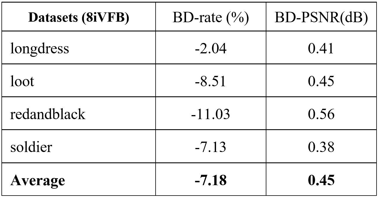
The rate-distortion performance is shown in Fig. 2. The bitrate is measured as bit per input point (bpip) and the distortion is evaluated using D1 measurement which computes the point-to-point distance between the original point cloud and the reconstructed point cloud. D1-PSNR is presented. Fig. 2 shows that the proposed method outperforms the other schemes. The measurement in terms of the Bjontegarrd metric is summarized in Table I to Table IV. The BD-rate and the BD-PSNR with respect to G-PCC is reported in Table I. On average, the proposed method gains 87.31% BD-rate reduction. Compared to V-PCC, Table II reports that the proposed method achieves 34.72% BD-rate reduction. Compared with the two learning-based schemes PCGCV1 and PCGCV2, the average BD-rate reductions are 35.83% and 4.4%, respectively. PCGCV1 is based on VAE architecture while the proposed method uses ANF. The superiority of the proposed method to PCGCV1 indicates that the latent in the proposed method better captures the input information. PCGCV2 uses a multi-scale design and both the downscaled latent and the skeleton octree are encoded. Even if the proposed method is not built upon a multi-scale design, it still has comparable performance.
To understand the improvement brought by the hierarchical FL, Fig. 2 shows also the performance of the proposed scheme without the hierarchical FL. Table V list the corresponding BD-rate and BDP-PSNR. From these results, the gains brought by the hierarchical FL is validated.
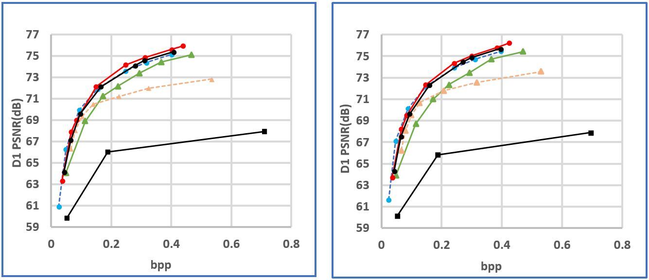
(a) longdress (b) loot
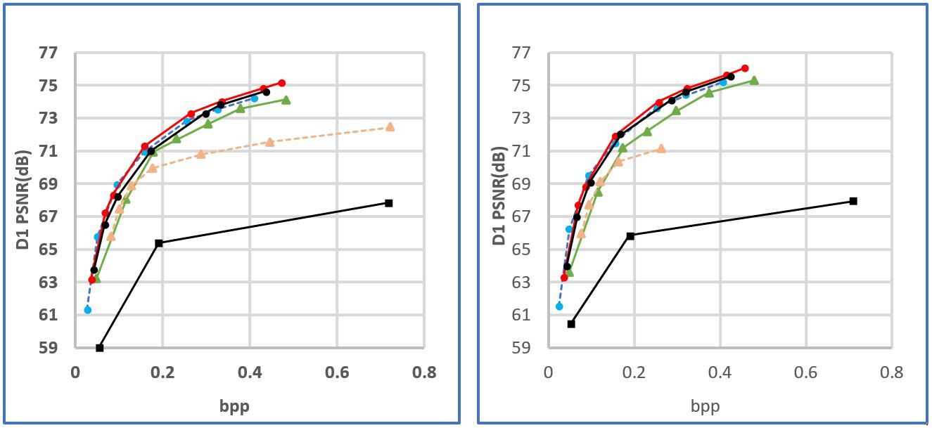
(c) redanblack (d) soldier

Fig. 4. R-D performance of the proposed method.
TABLE I. Bjontegarrd gains w.r.t G-PCC
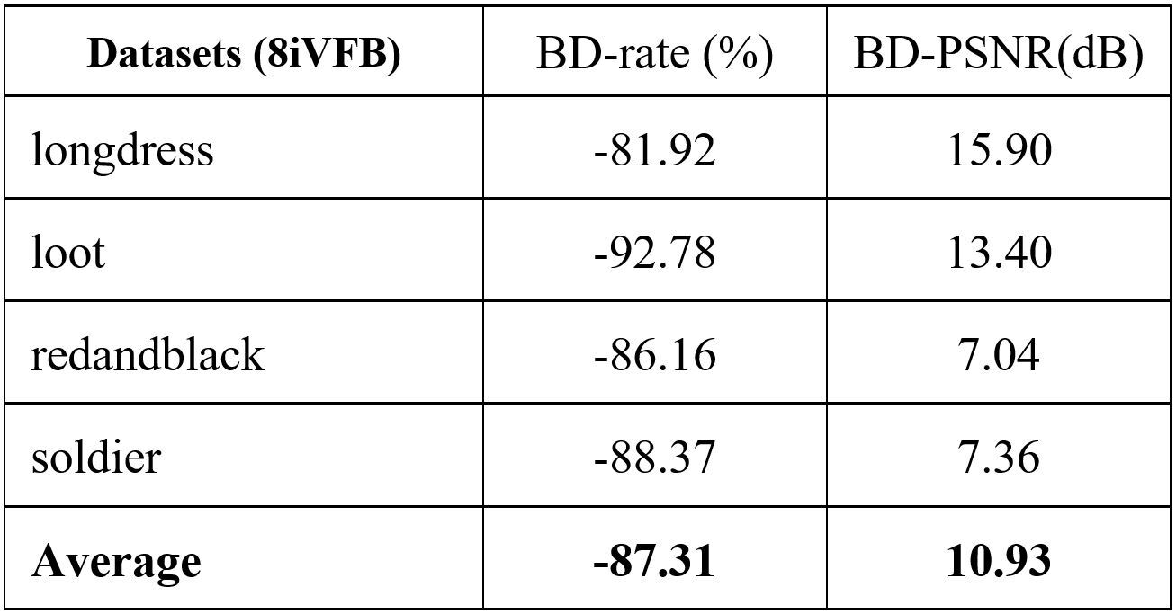
TABLE II. Bjontegarrd gains w.r.t V-PCC
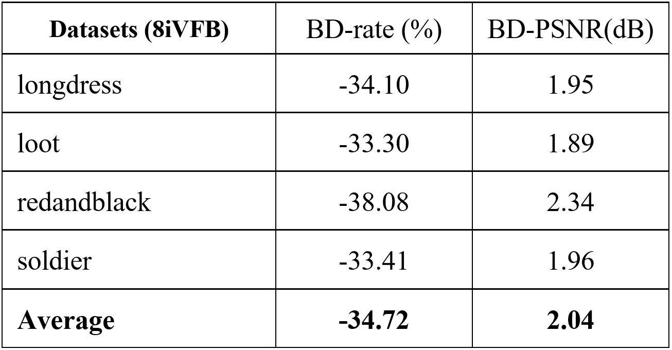
TABLE III. Bjontegarrd gains w.r.t PCGCv1 [11]
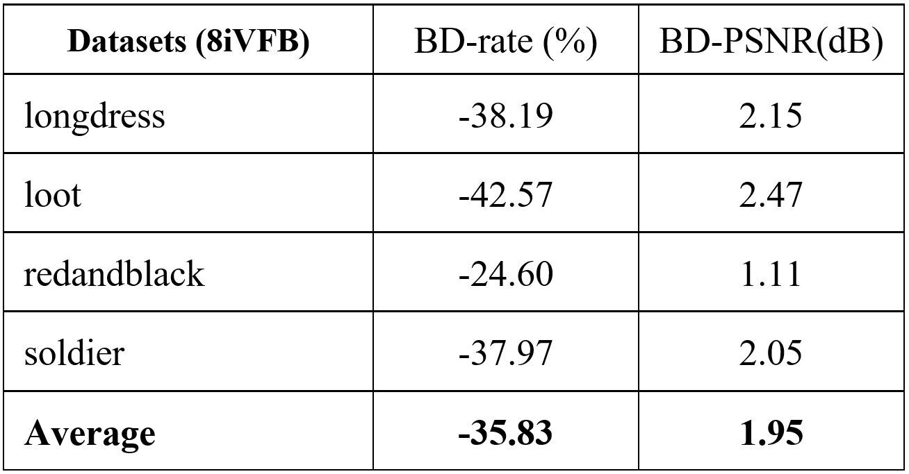
TABLE IV. Bjontegarrd gains w.r.t PCGCv2 [12]
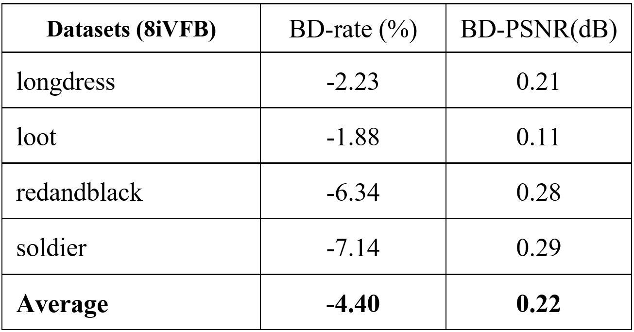
TABLE V. Bjontegarrd gains w.r.t without hierarchical FL
